Project page (Mildenhall et al): https://www.matthewtancik.com/nerf

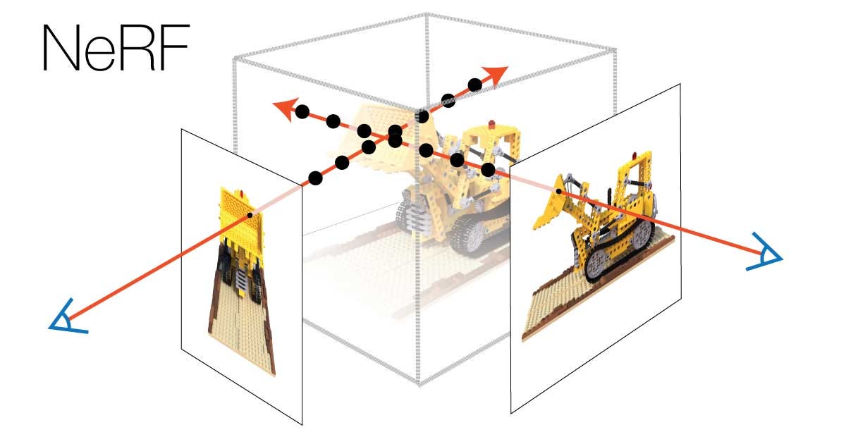
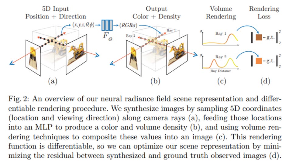
Neural Radiance Fields (NeRFs), implemented in a paper by a Berkeley research team in 2020, is a revolutionary method of displaying 3D objects and scenes given images and videos as training data. Instead of using 3D point clouds or meshes like photogrammetry and forward rendering methods, the scanned scenes and objects are transformed from a 5D coordinate (x, y, z, theta, phi) to a density and radiance output that is view dependent. This means that when a NeRF is generated given an array of camera images or videos of a scene, depending on the view of your camera traversing the scene, the rendered image is as if the camera was in the scene.

Understanding NeRFs

On a high level, NeRFs could be considered a volumetric representation of a pre-rendered scene. An important concept to know about is the image plane:

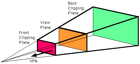
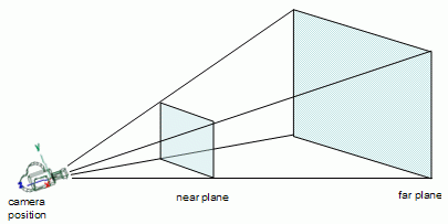
Given a camera, the image plane is the 2D projection of a 3D scene onto MxN pixels. If you take a picture with a camera, the image plane is the image that you get. Depending on your lens settings, such as focal length and sensor size, the image plane will change. In camera lenses, the range of changes and focal distances is shown in the camera’s frustum:

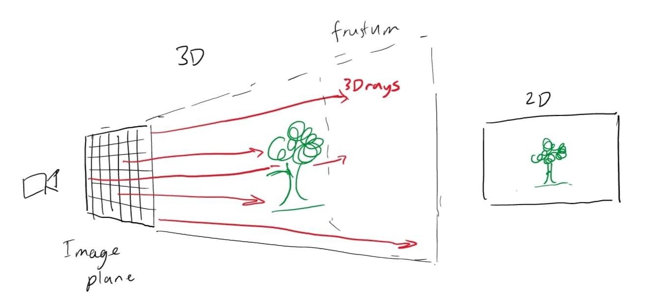
NeRFs use these image planes to actually render the scenes onto the 2D scene by inputting the camera position (x, y, z) and the viewing angle (theta, phi) into a function, where then the RGB color and density of each RGB pixel is computed and output onto the image plane through ray marching through the 3D space (explained a bit later). This is why NeRFs can provide view-dependent representations of the 3D planes.

To generate a NeRF, the model needs to know 1) the volumetric data (3D points of the 3D space) 2) the function F_Θ : (x, d) → (c, σ) to render the corresponding color and density at each viewing angle and position. The training only requires the images, the corresponding camera poses, intrinsic parameters, and the scene bounds.

To train the NeRF, the training data of RGB images with corresponding metadata about the camera’s position and rotation at each point is input to a multilayer perception network. Given a 2D image and the camera’s known properties, 3D rays can be constructed at every pixel of the image plane; therefore, at every single image, there are 3D rays that show all of the lines of sight on the image plane.

The model then randomly samples 3D points given these 3D rays from different images around the scene and inputs them into this function: F_Θ : (x, d) → (c, σ)

The input is 5D:

x → the 3D location of a voxel <x,y,z>

d → the viewing direction <theta, phi>

and the output is:

c → (r, g, b) color

sigma → volume density.

What this function is doing is grabbing the respective 3D voxel’s color and density (the opacity) given the camera’s viewing angle. A voxel is an infinitesimally small 3D cube in space. To evaluate this function’s weights, the output at rendered views across multiple views is compared to the ground truth 2D views. The loss is calculated with a total squared error between the rendered and true pixel colors. Using gradient descent for the MLP function, the weights Θ are optimized to map each 5D input coordinate to the corresponding volume density and directional emitted color of a 3D space. From the paper:

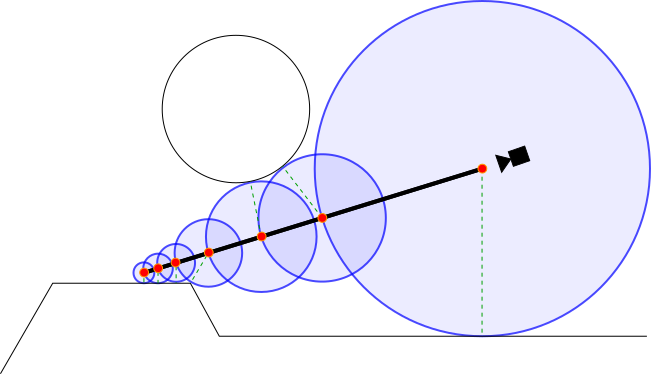
To have the representation be multiview consistent, the density is calculated relative to only the location x, while the color is calculated with the viewing angle included. The MLP outputs sigma and a 256-dimensional feature vector after passing through a 3D coordinate x with 8 fully connected layers. The feature vector is concatenated with the camera ray’s viewing direction and outputs a view-dependent RGB color. One thing to note is that this space is continuous → there isn’t a discrete “point cloud” the function is iterating across. This allows for very strong applications in providing accurate 3D representations without weird interpolation between views or an extremely extensive training set. However, to understand what c and sigma are actually modeling in the 3D space, and how NeRFs can render the 3D scenes, consider (source):

Each voxel has its color and density value according to the ray from a certain camera view, modeled as circles along a ray in the above image. If the voxel is in free space, the density would be close to 0. However, if the voxel represents an object, the density would be higher, and we could see the color in the rendered 2D image. To render the 2D image, rays from the camera perform ray marching, which is where along each step of the ray, a sine distance function is calculated to find the distance to the nearest object (voxel with a density above a certain threshold). This calculation continues down the ray until the distance is below a certain threshold. By sampling the radiance function along the ray, the model can determine the density and color of the pixel. By continuously doing this each iteration with randomly selected points, views, and rays, the model can improve its function weights.

To render the volume with the radiance field, the volume density is calculated simply with sigma(x) outputs the probability of a ray terminating at a particle at location x (density from ray marching). The color is calculated a bit more complexly:

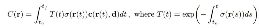
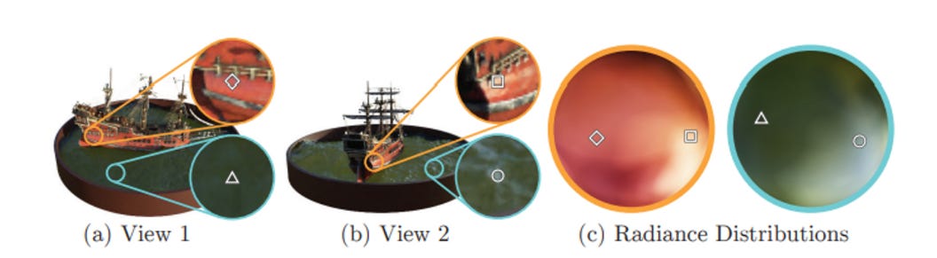
C(r) is the expected color of the camera ray, given that the ray is modeled r(t) = o + td, where the ray has near and far bounds tn and tf. T(t) is the accumulated transmittance (the probability that the ray travels from tn to tf without hitting another particle). The color is then the integral of the transmittance, density, and color at point t (between tn and tf) at viewing angle d. To estimate this continuous integral, the model uses a deterministic quadrature, where the MLP only queries at a discrete set of locations. However, the scene is still continuous because the MLP is evaluated at continuous locations. Below is a graphic from the paper which visualizes the view-dependent radiance.

An interesting thought is that light sources and rays in these NeRF representations are not actually rays as we may think in 3D rendering — we are only looking at the radiance off of objects, with light only changing the effect of the pixels like a 2D layer.

To improve the convergence, the team then uses positional encoding and hierarchical volume sampling. In some areas of high frequency, the MLP function performs poorly; by mapping x and d to a higher dimensional space, the MLP could more easily approximate a higher frequency function. Additionally, sampling N query points along a camera ray are inefficient since there are areas of free space and occluded regions that are still sampled repeatedly but do not really contribute to the rendered image. By optimizing a “coarse” and “fine” network, the network can produce a more informed sampling of points along each ray where samples are biased towards more relevant parts of the volume, which includes detailed and visible content.

Uses of NeRFs

The main use case of NeRFs currently is in robotics and in 3D asset generation for games, renderings, and films. Since NeRFs are continuous (as opposed to photogrammetry and 3D scanning which is discrete and cannot really do scenes well), the ability for flexible and accurate renders from different viewpoints provides great value to generating graphics from 2D inputs.

Luma AI is one of the leading startups working with NeRFs, optimizing a lot of the processes, reducing clouds, and providing NeRFs as assets for game engines like Unity and Unreal. Their API allows for very accurate and quick NeRFs given a few images or a video of a static environment and also has demos where one could bind game asset functions to generated NeRFs of objects. With the unique aspect of view-dependent rendering, one could import a NeRF to an engine like Unreal and use inverse rendering or light objects to simulate ray tracing on game objects. In the NVIDIA library Instant NGP (an optimized training for NeRFs), one could export a NeRF as a .glb or .obj file for input into Blender. I’m imagining Luma does it similarly, where the density of the 3D field is used as a way to render the objects as meshes, and the colors of the material could be estimated through the C(r) function (would love to investigate more on this entire process further).

The added benefit of a high-definition volumetric understanding of the environment helps a lot with robotics, embodied AI, and computer vision applications. I will go over several papers in a future post, but currently, researchers have embedded CLIP embeddings into NeRFs (LERF and CLIP-NeRF) as well as performed even better object detection and segmentation than in 2D images due to the density information (NeRF-SOS, NeRF-RPN). Additionally, the original team behind NeRFs has created NeRF Studio, an intuitive API and editor for creating NeRFs. I highly suggest taking a look at Luma AI’s Twitter and some of these papers to see what people are making with NeRFs.

Neural Radiance Fields have opened up exciting new possibilities for rendering 3D scenes and objects with incredible detail and accuracy. With the ability to generate highly realistic images from just a few input images or videos, NeRFs are transforming the fields of computer graphics, computer vision, and beyond. It’s pretty clear that NeRFs are poised to play a major role in shaping the future of digital imaging and visualization.